4.2. Example 1 - SXD+32 Point Source - Using the “reduce” command line

In this example, we will reduce the GNIRS crossed-dispersed observation of a supernova type II 54 days after explosion using the “reduce” command that is operated directly from the unix shell. Just open a terminal and load the DRAGONS conda environment to get started.

This cross-dispersed observation uses the 32 l/mm grating, the short-blue camera, and the 0.675 arcsec slit. The dither pattern is the standard ABBA repeated 5 times.

4.2.1. The dataset

If you have not already, download and unpack the tutorial’s data package. Refer to Downloading tutorial datasets for the links and simple instructions.

The dataset specific to this example is described in:

Example 1 - Datasets description

Here is a copy of the table for quick reference.

Science	N20170113S0146-165
Science flats	N20170113S0168-183
Pinholes	N20170113S0569-573
Science arcs	N20170113S0166-167
Telluric	N20170113S0123-138
BPM	bpm_20121101_gnirs_gnirsn_11_full_1amp.fits

4.2.2. Configuring the interactive interface

In ~/.dragons/, add the following to the configuration file dragonsrc:

[interactive]
browser = your_preferred_browser

The [interactive] section defines your preferred browser. DRAGONS will open the interactive tools using that browser. The allowed strings are “safari”, “chrome”, and “firefox”.

4.2.3. Set up the Local Calibration Manager

Important

Remember to set up the calibration service.

Instructions to configure and use the calibration service are found in Setting up the Calibration Service, specifically the these sections: The Configuration File and Usage from the Command Line.

We recommend that you clean up your working directory (playground) and start a fresh calibration database (caldb init -w) when you start a new example.

4.2.4. Create file lists

This data set contains science and calibration frames. For some programs, it could contain different observed targets and different exposure times depending on how you like to organize your raw data.

The DRAGONS data reduction pipeline does not organize the data for you. You have to do it. However, DRAGONS provides tools to help you with that.

The first step is to create input file lists. The tool “dataselect” helps. It uses Astrodata tags and descriptors to select the files and send the filenames to a text file that can then be fed to “reduce”. (See the Astrodata User Manual for information about Astrodata and for a list of descriptors.)

First, navigate to the playground directory in the unpacked data package:

cd <path>/gnirsxd_tutorial/playground

4.2.4.1. A list for the flats

The GNIRS XD flats are obtained using two different lamps to ensure that each order is illuminated at a sufficient level. The software will stack each set and automatically assemble the orders into a new flat with all orders well illuminated. You will use “dataselect” to select all the flats associated with our science observation.

dataselect ../playdata/example1/*.fits --tags FLAT -o flats.lis

4.2.4.2. A list for the pinholes

The orders are significantly slanted and curved on the detector. While the edges of the orders in the processed flat can be used to determine the position of each order, the pinholes observations lead to a more accurate model of the order positions. The pinholes are taken in the same configuration as for the science.

dataselect ../playdata/example1/*.fits --tags PINHOLE -o pinholes.lis

4.2.4.3. A list for the arcs

The GNIRS cross-dispersed arcs were obtained at the end of the science observation. Often two are taken. If we decide to use both, they will be stacked.

dataselect ../playdata/example1/*.fits --tags ARC -o arcs.lis

4.2.4.4. A list for the telluric

DRAGONS does not recognize the telluric star as such. This is because, at Gemini, the observations are taken like science data and the GNIRS headers do not explicitly state that the observation is a telluric standard. In most cases, the observation_class descriptor can be used to differentiate the telluric from the science observations, along with the rejection of the CAL tag to reject flats and arcs.

dataselect ../playdata/example1/*.fits --xtags=CAL --expr='observation_class=="partnerCal"' -o telluric.lis

4.2.4.5. A list for the science observations

The science observations can be selected from the “observation class” science. This is how they are differentiated from the telluric standards which are most often set to partnerCal.

If we had multiple targets, we would need to split them into separate lists. To inspect what we have we can use dataselect and showd together.

dataselect ../playdata/example1/*.fits --expr='observation_class=="science"' | showd -d object

--------------------------------------------------
filename                                    object
--------------------------------------------------
../playdata/example1/N20170113S0146.fits   DLT16am
../playdata/example1/N20170113S0147.fits   DLT16am
../playdata/example1/N20170113S0148.fits   DLT16am
...
../playdata/example1/N20170113S0163.fits   DLT16am
../playdata/example1/N20170113S0164.fits   DLT16am
../playdata/example1/N20170113S0165.fits   DLT16am

Here we only have one object from the same sequence. If we had multiple objects we could add the object name in the expression.

dataselect ../playdata/example1/*.fits --expr='observation_class=="science" and object=="DLT16am"' -o sci.lis

4.2.5. Bad Pixel Mask

The bad pixel masks (BPMs) are handled as calibrations. They are downloadable from the archive instead of being packaged with the software. They are automatically associated like any other calibrations. This means that the user now must download the BPMs along with the other calibrations and add the BPMs to the local calibration manager.

See Get the BPMs in Tips and Tricks to learn about the various ways to get the BPMs from the archive.

To add the static BPM included in the data package to the local calibration database:

caldb add ../playdata/example1/bpm*.fits

4.2.6. Master Flat Field

GNIRS XD flat fields are normally obtained at night along with the observation sequence to match the telescope and instrument flexure. The processed flat is constructed from two sets of stacked lamp-on flats, each illuminated differently to ensure that all orders in the reassembled flat are well illuminated. You do not have to worry about the details, as long as you pass the two sets of raw flats as input to the reduce command, the software will take care of the assembly.

The processed flat will also contain the illumination mask that identify the location of the illuminated areas in the array, ie, where the orders are located.

reduce @flats.lis

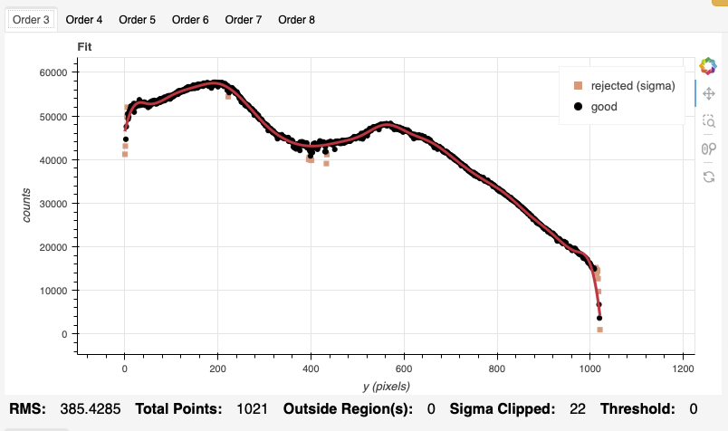
In interactive mode, you can inspect the fit for each order by selecting the tabs above the plot.

Note that you are not required to run in interactive mode, but you might want to if flat fielding is critical to your program.

reduce @flats.lis -p interactive=True

The interactive tools are introduced in section Interactive tools.

4.2.7. Processed Pinholes - Rectification

The pinholes are used to determine the rectification of the slanted and curved orders. A pinhole observation looks like this:

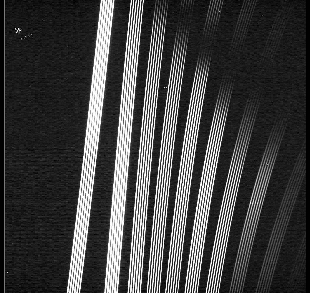
The rectification model is calculated by tracing the dispersed image of each pinhole in each order.

reduce @pinholes.lis

4.2.8. Processed Arc - Wavelength Solution

Obtaining the wavelength solution for GNIRS cross-dispersed data can be a complicated topic. The quality of the results and what to use depend greatly on the wavelength regime and the grating.

Our configuration in this example is cross-dispersed with short-blue camera and the 32 l/mm grating. This configuration generally has a sufficient number of lines available in all the orders.

For more information about wavelength calibration, see the Wavelength Calibration Guide for GNIRS XD.

The illumination mask will be obtained from the processed flat. The processed pinhole will provide the distortion correction.

reduce @arcs.lis

The primitive determineWavelengthSolution, used in the recipe, has an interactive mode. To activate the interactive mode:

reduce @arcs.lis -p interactive=True

The interactive tools are introduced in section Interactive tools.

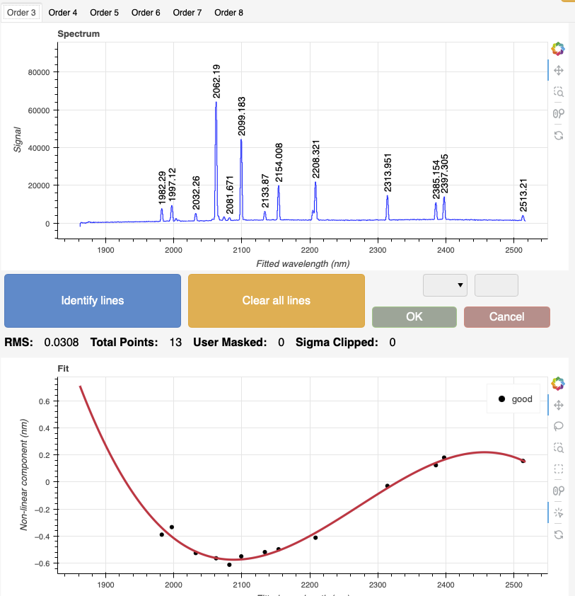
Each order can be inspected individually by selecting the tabs above the plot.

The general shape of the fit for each order should look like this:

4.2.9. Telluric Standard

The telluric standard observed before the science observation is “hip 17030”. The spectral type of the star is A0V.

To properly calculate and fit a telluric model to the star, we need to know its effective temperature. To properly scale the sensitivity function (to use the star as a spectrophotometric standard), we need to know the star’s magnitude. Those are inputs to the fitTelluric primitive.

The default effective temperature of 9650 K is typical of an A0V star, which is the most common spectral type used as a telluric standard. Different sources give values between 9500 K and 9750 K and, for example, Eric Mamajek’s list “A Modern Mean Dwarf Stellar Color and Effective Temperature Sequence” (https://www.pas.rochester.edu/~emamajek/EEM_dwarf_UBVIJHK_colors_Teff.txt) quotes the effective temperature of an A0V star as 9700 K. The precise value has only a small effect on the derived sensitivity and even less effect on the telluric correction, so the temperature from any reliable source can be used. Using Simbad, we find that the star has a magnitude of K=9.244.

Instead of typing the values on the command line, we will use a parameter file to store them. In a normal text file (here we name it “hip17030.param”), we write:

-p
fitTelluric:bbtemp=9700
fitTelluric:magnitude='K=9.244'

Then we can call the reduce command with the parameter file. The telluric fitting primitive can be run in interactive mode.

Note that the data are recognized by Astrodata as normal GNIRS cross-dispersed science spectra. To calculate the telluric correction, we need to specify the telluric recipe (-r reduceTelluric), otherwise the default science reduction will be run.

reduce @telluric.lis -r reduceTelluric @hip17030.param -p fitTelluric:interactive=True

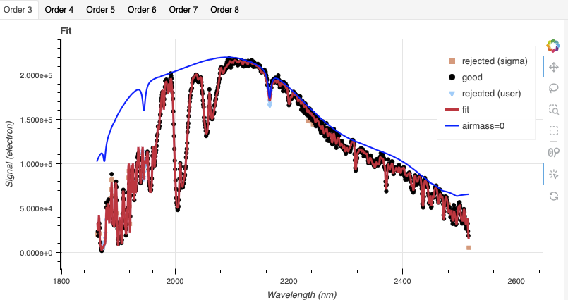
The fit for Order 3 looks like this:

4.2.10. Science Observations

The science target is a supernova type II 54 days after explosion. The sequence is 5 ABBA dither pattern. DRAGONS will flatfield, wavelength calibrate, subtract the sky, stack the aligned spectra, extract the source, and finally remove telluric features and flux calibrate.

Note

In this observation, there is only one real source to extract. If there were multiple sources in the slit, regardless of whether they are of interest to the program or not, DRAGONS will locate them, trace them, and extract them automatically. Each extracted spectrum is stored in an individual extension in the output multi-extension FITS file.

This is what one raw image looks like.

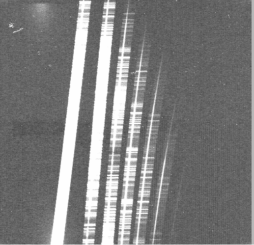
What you see are from left to right the cross-dispersed orders, from Order 3 to Order 8. The short horizontal features are sky lines. The “vertical lines” are the dispersed science target in each order. In the raw data, the red end is at the bottom and blue at the top. This will be reversed when the data is resampled and the distortion corrected and wavelength calibration are applied.

With all the calibrations in the local calibration manager, one only needs to call reduce on the science frames to get an extracted spectrum.

reduce @sci.lis

To run the reduction with all the interactive tools activated, set the interactive parameter to True.

reduce @sci.lis -p interactive=True

---

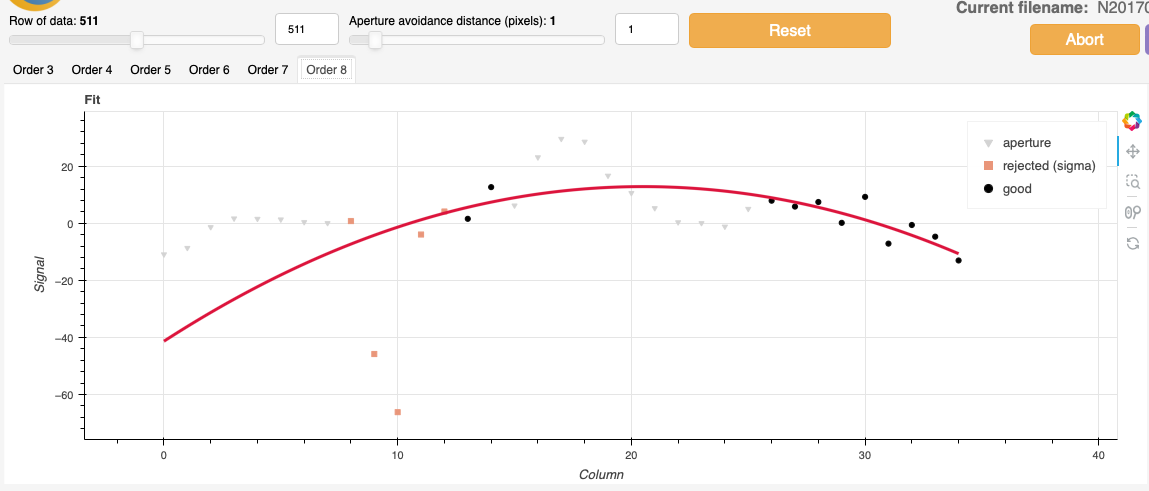
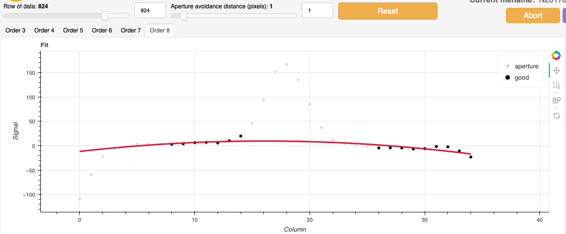
skyCorrectFromSlit

At the skyCorrectFromSlit step, you will notice that the fit for Order 8 is not very good. The row being sampled is in the middle of the image. If you look at the raw image, you will see that there is not much signal for Order 8 in the middle row. Increase the row number (the data has been resampled and flipped at this point) using the slider at the top-left of the tool and you will see that when there is signal the fit is good. Bottom line: where there is signal, the fit is good, that’s what we wish to verify.

telluricCorrect

When you get to the telluricCorrect step, you can experiment with the shift between the telluric standard and the target. Both need to be well aligned in wavelength to optimize the correction. In this case, we find that a shift of 0.55 pixels significantly improves the correction.

---

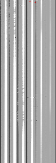
A section of 2D spectrum before extraction is shown on the right, with blue wavelengths at the bottom and the red-end at the top. Note that each order has been rectified and is being stored in separate extensions in the MEF file. Here they are displayed together, side by side. (reduce -r display N20170113S0146_2D.fits, launch DS9 first.)

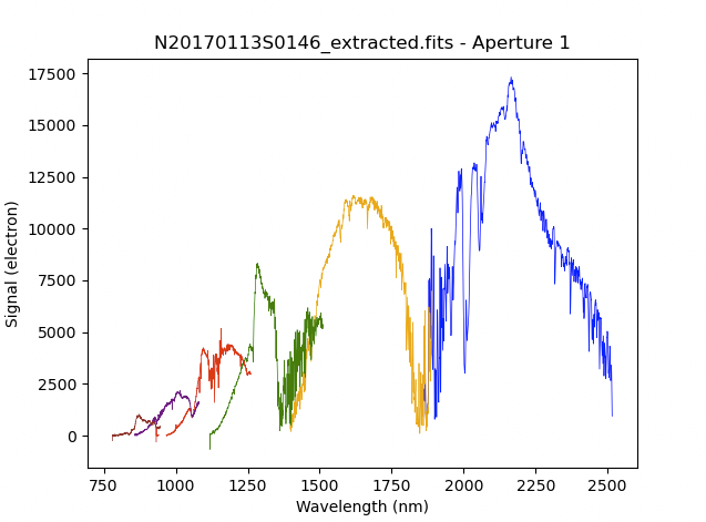
Each order is extracted separately and stored in separate extensions in the MEF file. The 1D extracted spectrum before telluric correction or flux calibration, obtained by adding the option -p extractSpectra:write_outputs=True to the reduce call. You can plot all the orders on a common plot with dgsplot. (The --thin option simply plots a thinner line than the default width.)

dgsplot N20170113S0146_extracted.fits 1 --thin

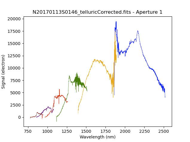
The 1D extracted spectrum after telluric correction but before flux calibration, obtained with -p telluricCorrect:write_outputs=True, looks like this.

dgsplot N20170113S0146_telluricCorrected.fits 1 --thin

And the final spectrum, corrected for telluric features and flux calibrated.

dgsplot N20170113S0146_1D.fits 1 --thin

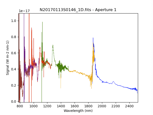
In the final spectrum, the orders are remain separated. Here they are simply plotted one after the other on a common plot.

If you need to stitch the order and stack the common wavelength ranges, you can use the combineOrders primitive.

reduce -r combineOrders N20170113S0146_1D.fits

dgsplot N20170113S0146_ordersCombined.fits 1 --thin