5.2. Example 2 - SXD+111 Point Source - Using the “reduce” command line

In this example, we will reduce the GNIRS crossed-dispersed observation of an erupting recurrent nova using the “reduce” command that is operated directly from the unix shell. Just open a terminal and load the DRAGONS conda environment to get started.

This cross-dispersed observation uses the 111 l/mm grating, the short-blue camera and the 0.3 arcsec slit. The dither pattern is the standard ABBA, one set for each of the three central wavelength settings. The results from the three wavelength settings will be stitched together at the end.

5.2.1. The dataset

If you have not already, download and unpack the tutorial’s data package. Refer to Downloading tutorial datasets for the links and simple instructions.

The dataset specific to this example is described in:

Example 1 - Datasets description

Here is a copy of the table for quick reference.

Science	N20191013S0006-09 (1.55 ${\mu}$ m) N20191013S0010-13 (1.68 ${\mu}$ m) N20191013S0014-17 (1.81 ${\mu}$ m)
Science flats	N20191013S0036-51 (1.55 ${\mu}$ m) N20191013S0054-69 (1.68 ${\mu}$ m) N20191013S0072-87 (1.81 ${\mu}$ m)
Pinholes	None available
Science arcs	N20191013S0034-35 (1.55 ${\mu}$ m) N20191013S0052-53 (1.68 ${\mu}$ m) N20191013S0070-71 (1.81 ${\mu}$ m)
Telluric	N20191013S0022-25 (1.55 ${\mu}$ m) N20191013S0026-29 (1.68 ${\mu}$ m) N20191013S0030-33 (1.81 ${\mu}$ m)
BPM	bpm_20121101_gnirs_gnirsn_11_full_1amp.fits

5.2.2. Configuring the interactive interface

In ~/.dragons/, add the following to the configuration file dragonsrc:

[interactive]
browser = your_preferred_browser

The [interactive] section defines your preferred browser. DRAGONS will open the interactive tools using that browser. The allowed strings are “safari”, “chrome”, and “firefox”.

5.2.3. Set up the Local Calibration Manager

Important

Remember to set up the calibration service.

Instructions to configure and use the calibration service are found in Setting up the Calibration Service, specifically the these sections: The Configuration File and Usage from the Command Line.

We recommend that you clean up your working directory (playground) and start a fresh calibration database (caldb init -w) when you start a new example.

5.2.4. Create file lists

This data set contains science and calibration frames. For some programs, it could contain different observed targets and different exposure times depending on how you like to organize your raw data.

The DRAGONS data reduction pipeline does not organize the data for you. You have to do it. However, DRAGONS provides tools to help you with that.

The first step is to create input file lists. The tool “dataselect” helps. It uses Astrodata tags and descriptors to select the files and send the filenames to a text file that can then be fed to “reduce”. (See the Astrodata User Manual for information about Astrodata and for a list of descriptors.)

First, navigate to the playground directory in the unpacked data package:

cd <path>/gnirsxd_tutorial/playground

5.2.4.1. Three lists for the flats

The GNIRS XD flats are obtained using two different lamps to ensure that each order is illuminated at a sufficient level. The software will stack each set and automatically assemble the orders into a new flat with all orders well illuminated.

The particularily of this dataset is that there are three central wavelength settings that each need to be reduced separately.

You will use “dataselect” to select each set of flats associated with the configurations used for the science observations.

But first, to see which central wavelengths have been used, run showd on the flats.

dataselect ../playdata/example2/*.fits --tags FLAT | showd -d central_wavelength

-------------------------------------------------------------
filename                                   central_wavelength
-------------------------------------------------------------
../playdata/example2/N20191013S0036.fits             1.55e-06
../playdata/example2/N20191013S0037.fits             1.55e-06
...
../playdata/example2/N20191013S0054.fits             1.68e-06
../playdata/example2/N20191013S0055.fits             1.68e-06
...
../playdata/example2/N20191013S0072.fits             1.81e-06
../playdata/example2/N20191013S0073.fits             1.81e-06

dataselect ../playdata/example2/*.fits --tags FLAT --expr='central_wavelength==1.55e-6' -o flat155.lis
dataselect ../playdata/example2/*.fits --tags FLAT --expr='central_wavelength==1.68e-6' -o flat168.lis
dataselect ../playdata/example2/*.fits --tags FLAT --expr='central_wavelength==1.81e-6' -o flat181.lis

Note that we have downloaded only the October data from that program. If the September data were also in our raw data directory, we would have to add a date constraint to the expression, like this:

dataselect ../playdata/example2/*.fits --tags FLAT --expr='central_wavelength==1.55e-6 and ut_date=="2019-10-13"' -o flatSep155.lis

5.2.4.2. A list for the pinholes

This program does not use a pinholes observation.

The orders in the cross-dispersed raw data are significantly slanted and curved on the detector. A pinhole would trace that curvature.

However, the edges of the orders in the processed flat can be used to determine the position of each order, the pinholes observations simply lead to a more accurate model of the order positions and of the spatial distortion component.

We do not have pinholes, therefore all steps related to pinholes, their creation and their usage will be skipped in this tutorial.

If you had pinholes, you would select them like for the flats above using “PINHOLE” instead of “FLAT”.

5.2.4.3. Three lists for the arcs

The GNIRS cross-dispersed arcs were obtained between the telluric and the science observation. Often two are taken for each configuration. If we decide to use both, they will be stacked.

Here, like for the flats, we need to create a list for each of the three configurations.

dataselect ../playdata/example2/*.fits --tags ARC --expr='central_wavelength==1.55e-6' -o arc155.lis
dataselect ../playdata/example2/*.fits --tags ARC --expr='central_wavelength==1.68e-6' -o arc168.lis
dataselect ../playdata/example2/*.fits --tags ARC --expr='central_wavelength==1.81e-6' -o arc181.lis

5.2.4.4. Three lists for the telluric

DRAGONS does not recognize the telluric star as such. This is because, at Gemini, the observations are taken like science data and the GNIRS headers do not explicitly state that the observation is a telluric standard. In most cases, the observation_class descriptor can be used to differentiate the telluric from the science observations, along with the rejection of the CAL tag to reject flats and arcs. Telluric stars will be observed under the partnerCal or progCal classes, the science observation under the science class.

dataselect ../playdata/example2/*.fits --xtags=CAL --expr='observation_class!="science" and central_wavelength==1.55e-6' -o tel155.lis
dataselect ../playdata/example2/*.fits --xtags=CAL --expr='observation_class!="science" and central_wavelength==1.68e-6' -o tel168.lis
dataselect ../playdata/example2/*.fits --xtags=CAL --expr='observation_class!="science" and central_wavelength==1.81e-6' -o tel181.lis

5.2.4.5. A list for the science observations

The science observations can be selected from the “observation class” science. This is how they are differentiated from the telluric standards which are set to partnerCal or progCal.

We already know that we have multiple central_wavelength settings and that we will need a list of each.

If we had multiple targets, we would need to split them into separate lists. To inspect what we have we can use dataselect and showd together.

dataselect ../playdata/example2/*.fits --expr='observation_class=="science"' | showd -d object,central_wavelength

-------------------------------------------------------------------------
filename                                      object   central_wavelength
-------------------------------------------------------------------------
../playdata/example2/N20191013S0006.fits   V3890 Sgr             1.55e-06
../playdata/example2/N20191013S0007.fits   V3890 Sgr             1.55e-06
../playdata/example2/N20191013S0008.fits   V3890 Sgr             1.55e-06
../playdata/example2/N20191013S0009.fits   V3890 Sgr             1.55e-06
../playdata/example2/N20191013S0010.fits   V3890 Sgr             1.68e-06
../playdata/example2/N20191013S0011.fits   V3890 Sgr             1.68e-06
../playdata/example2/N20191013S0012.fits   V3890 Sgr             1.68e-06
../playdata/example2/N20191013S0013.fits   V3890 Sgr             1.68e-06
../playdata/example2/N20191013S0014.fits   V3890 Sgr             1.81e-06
../playdata/example2/N20191013S0015.fits   V3890 Sgr             1.81e-06
../playdata/example2/N20191013S0016.fits   V3890 Sgr             1.81e-06
../playdata/example2/N20191013S0017.fits   V3890 Sgr             1.81e-06

Here we only have one object from the same sequence. If we had multiple objects we could add the object name in the expression.

dataselect ../playdata/example2/*.fits --expr='observation_class=="science" and central_wavelength==1.55e-6 and object=="V3890 Sgr"' -o sci155.lis
dataselect ../playdata/example2/*.fits --expr='observation_class=="science" and central_wavelength==1.68e-6 and object=="V3890 Sgr"' -o sci168.lis
dataselect ../playdata/example2/*.fits --expr='observation_class=="science" and central_wavelength==1.81e-6 and object=="V3890 Sgr"' -o sci181.lis

5.2.5. Bad Pixel Mask

The bad pixel masks (BPMs) are handled as calibrations. They are downloadable from the archive instead of being packaged with the software. They are automatically associated like any other calibrations. This means that the user now must download the BPMs along with the other calibrations and add the BPMs to the local calibration manager.

See Get the BPMs in Tips and Tricks to learn about the various ways to get the BPMs from the archive.

To add the static BPM included in the data package to the local calibration database:

caldb add ../playdata/example2/bpm*.fits

5.2.6. Master Flat Field

GNIRS XD flat fields are normally obtained at night along with the observation sequence to match the telescope and instrument flexure. The processed flat is constructed from two sets of stacked lamp-on flats, each exposed differently to ensure that all orders in the reassembled flat are well illuminated. You do not have to worry about the details, as long as you pass the two sets of raw flats as input to the reduce command, the software will take care of the assembly.

The processed flat will also contain the illumination mask that identify the location of the illuminated areas in the array, ie, where the orders are located. By tracing the edges of the illuminated areas, a rectification model is also calculated.

Each central wavelength settings must be reduced separately.

reduce @flat155.lis
reduce @flat168.lis
reduce @flat181.lis

It might be useful to run the flat reduction in interactive mode. Also, in this case, using -p normalizeFlat:grow=2 helps rejecting the pixels near the edge and ensure a smoother fit. You can play with the other parameters too.

reduce @flat155.lis -p interactive=True normalizeFlat:grow=2
reduce @flat168.lis -p interactive=True normalizeFlat:grow=2
reduce @flat181.lis -p interactive=True normalizeFlat:grow=2 normalizeFlat:niter=2

The interactive tools are introduced in section Interactive tools.

Note

In some data the “odd-even effect”, some noise pattern affecting odd and even rows differently cannot not be perfectly corrected. In those cases, you will see the black dots define two separated signal trace. Get the fit to trace the middle. In most cases, the effect in science and telluric data is removed during the flat fielding.

5.2.7. Processed Pinholes - Rectification

The pinholes are used to determine the rectification of the slanted and curved orders.

This program does not have pinholes associated with it. It is okay, the edges of the orders have been traced when the flats were reduced. This can be used for the rectification. The spatial axis is not as well sampled but depending on the science using just the edges from the flat can be sufficient.

Since the attachPinholeRectification step will have to be skipped for all the recipes that requests it, let’s save ourselves some typing and let’s put that instructions in an file that we can attach later to our reduce calls.

echo "-p attachPinholeRectification:skip_primitive=True" > nopinhole.param

If you had pinhole observation, just like the flats they would need to be reduced each configuration separately (eg. reduce @pinhole155.lis)

5.2.8. Wavelength Solution

Obtaining the wavelength solution for GNIRS cross-dispersed data can be a complicated topic. The quality of the results and whether to use arc lamp or sky lines depends greatly on the wavelength regime and the grating.

Caution

Do pay great attention to the wavelength calibration. It is critical to the telluric modelling. It can be particularly challenging with the 111 l/mm grating given the limited wavelength range each order covers.

Our configurations in this example is cross-dispersed with short-blue camera, the SXD prism, and the 111 l/mm grating. With this grating, each order covers only a short wavelength range. Some orders will not contain a sufficient number of lines from the arc lamp. In some cases, we will have to use the sky emission lines, or even the telluric absorption features to get an accurate enough wavelength solution for an order.

Note

The current software calculates a wavelength solution for each order separately. A “2D solution” that would use all the lines from all the orders together is not yet available.

5.2.8.1. Summary of the Technique for Science Quality

The wavelength calibration is critical to the telluric modelling. In fact, the best way to know which wavelength solutions work for each order and which ones do not is to run fitTelluric interactively and see if the modeling works well or not.

For quicklook results, you might not care to go through the trouble, but for a science quality product, you will have to go through the following steps.

For each central wavelength setting:

Produce a wavelength solution from the arc lamp.
Produce a wavelength solution from the sky emission lines in the science data.
Launch the telluric star reduction in interactive mode.

First using the arc lamp solution. Inspect each order. Identify which one works, which one does not.

Then using the sky lines solution. Inspect each order. Identify which one works, which one does not.

Piece together the best solutions for each order and add this “processed arc” to the calibration database.
Clean up the calibration database of the arc and sky lines solutions, leaving only the ones built during Step 4.

Later, you will be doing the “official” reduction of the telluric star and the reduction of the science target using the wavelength solution put together in step 4. It will be picked up automatically.

Hint

It is expected that for a set of H-band central wavelengths, like this case, sky emission lines will provide the most comprehensive coverage. It is not complete however and it will need to be complemented with arc lamp solutions.

5.2.8.2. Solution from the Arc Lamp

During the processing of the arc, the illumination mask and the rectification model will be obtained from the processed flat.

reduce @arc155.lis -p interactive=True @nopinhole.param
reduce @arc168.lis -p interactive=True @nopinhole.param
reduce @arc181.lis -p interactive=True @nopinhole.param

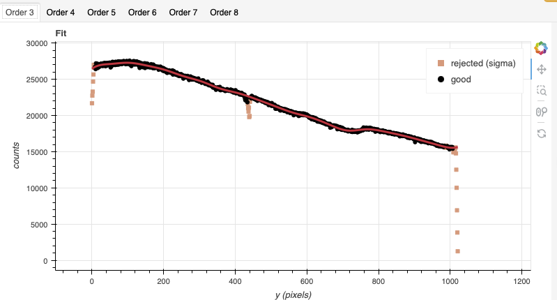
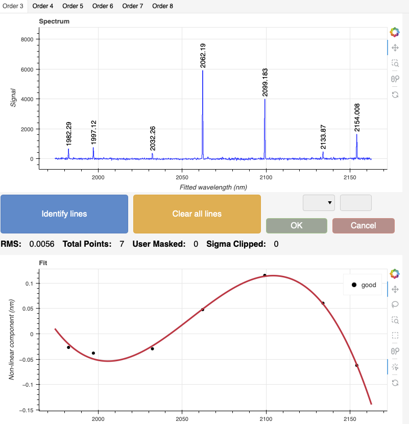
The interactive tools are introduced in section Interactive tools.

Each order can be inspected individually by selecting the tabs above the plot.

The general shape of the fit for each order should look like this:

Arc line identifications and fit for Order 3

While the solutions from the arc lamp are not so bad for central wavelength 1.55 and 1.68 ${\mu}$ m, they are quite bad in general for the 1.81 ${\mu}$ m setting.

5.2.8.3. Solution from Sky Emission Lines

If the exposure times are long enough, chances are that the OH and O₂ sky lines are your best bet to get a good solution in most orders at most H-band settings, especially if you do not need Order 7 and 8.

reduce -r makeWavecalFromSkyEmission @sci155.lis -p interactive=True @nopinhole.param
reduce -r makeWavecalFromSkyEmission @sci168.lis -p interactive=True @nopinhole.param
reduce -r makeWavecalFromSkyEmission @sci181.lis -p interactive=True @nopinhole.param

For the 1.55 ${\mu}$ m setting, beware that the automatic solution for Order 7 is completely wrong. Delete all the lines and identify them manually. Remember to set the fit order to 3 once you have identified a few lines. Order 8 has no solution since there are no lines. It will use an approximate linear solution to complete. We will not be using it anyway in this case since the arc solution for Order 8 is reasonable.

For the 1.68 ${\mu}$ m and 1.81 ${\mu}$ m settings, the solutions are generally good except for Order 8 where the lines needs to be added manually.

5.2.8.4. Verifying the Solutions with fitTelluric

We will verify the solutions we calculated above. We have:

Arc at 1.55 ${\mu}$ m	N20191013S0034_arc.fits
Arc at 1.68 ${\mu}$ m	N20191013S0052_arc.fits
Arc at 1.81 ${\mu}$ m	N20191013S0070_arc.fits
Sky lines at 1.55 ${\mu}$ m	N20191013S0006_arc.fits
Sky lines at 1.68 ${\mu}$ m	N20191013S0010_arc.fits
Sky lines at 1.81 ${\mu}$ m	N20191013S0014_arc.fits

We need to run fitTelluric with each one and assess the quality of the model for each order. We use the --user_cal option to override the automatic “proccessed arc” selection.

We need to use information about the star like the temperature and the magnitude. See the section about the modeling of the telluric below for more details. For now, create a file named hip94510.param with this content:

-p
fitTelluric:bbtemp=9700
fitTelluric:magnitude='K=6.754'

5.2.8.4.1. For 1.55 ${\mu}$ m

You can “Abort” fitTelluric when you are done with the inspection.

reduce @tel155.lis -r reduceTelluric --user_cal processed_arc:N20191013S0034_arc.fits -p fitTelluric:interactive=True @hip94510.param @nopinhole.param

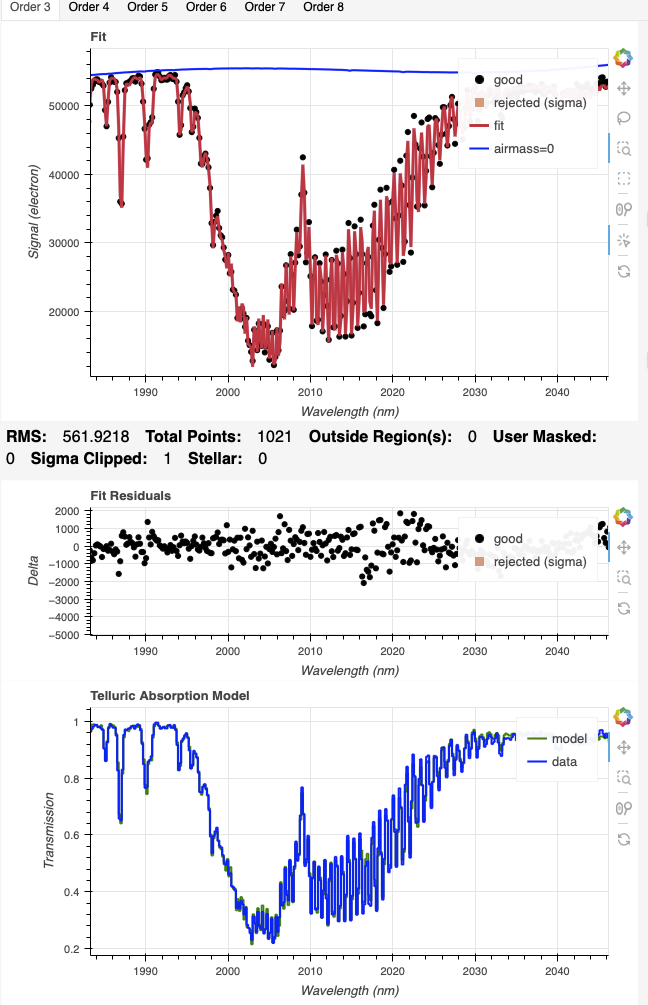
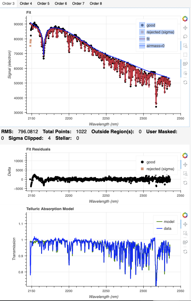
You will see that the “ringing” in the deep telluric features is well fit. Order 3 to 5, and Order 8 give a good result. In Order 6 and 7, the wavelength scale is clearly offset and the model is wrong.

reduce @tel155.lis -r reduceTelluric --user_cal processed_arc:N20191013S0006_arc.fits -p fitTelluric:interactive=True @hip94510.param @nopinhole.param

The ringing is not as well fit, if at all when using the solution from the sky lines. However, the fits for Order 6 and 7 are good.

CONCLUSION

For 1.55 ${\mu}$ m, use the arc solution for Order 3-5, 8, and the sky solution for Order 6 and 7.

Here are examples of what to look for. First for Order 3, we can see that the model follows the ringing quite well with the arc solution and not well at all with the sky solution, even after adjust the LSF scaling factor to match what is used for the arc solution (1.06).

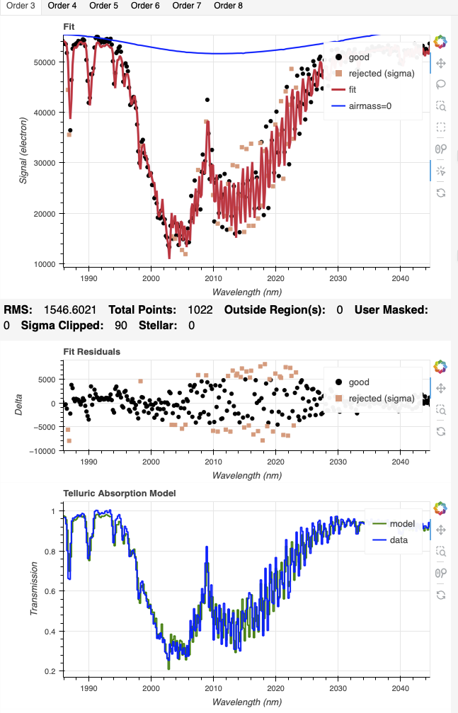
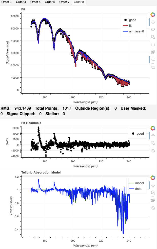
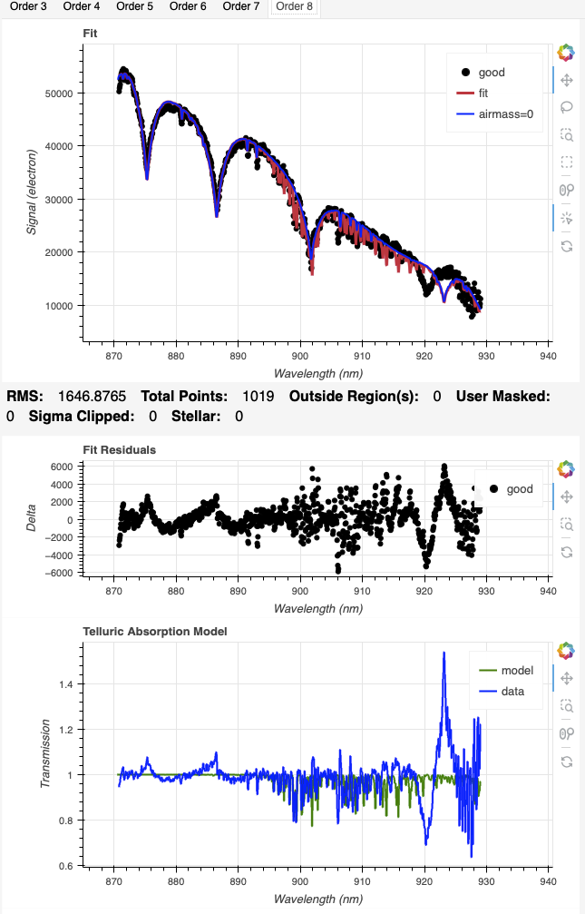
The second example is for Order 7, where the sky solution on the right is, while not perfect, clearly better.

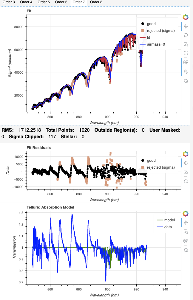
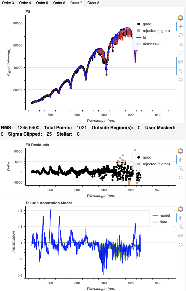
5.2.8.4.2. For 1.68 ${\mu}$ m

reduce @tel168.lis -r reduceTelluric --user_cal processed_arc:N20191013S0052_arc.fits -p fitTelluric:interactive=True @hip94510.param @nopinhole.param

The solutions from arc are reasonable for all orders. However, we will see that the sky lines are doing better for Orders 3-7.

reduce @tel168.lis -r reduceTelluric --user_cal processed_arc:N20191013S0010_arc.fits -p fitTelluric:interactive=True @hip94510.param @nopinhole.param

From the sky lines, Order 8 is not usable. But overall, the fit for the Orders are better than from the arc lamp solution.

CONCLUSION

For 1.68 ${\mu}$ m, use the arc solution for Order 8, and the sky solution for Orders 3 to 7.

While the differences can be obvious like for Order 8, some might be a little more subtle. For example, here we compare Order 3. The model calculated with the arc solution, on the left, is more noisy than the one with the sky solution on the right.

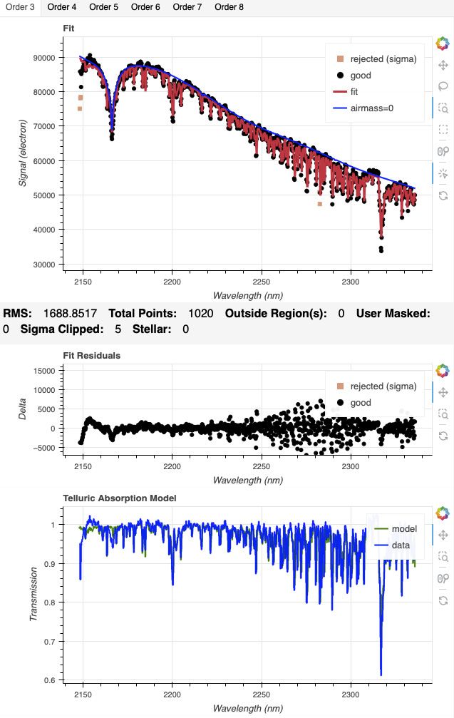
5.2.8.4.3. For 1.81 ${\mu}$ m

reduce @tel181.lis -r reduceTelluric --user_cal processed_arc:N20191013S0070_arc.fits -p fitTelluric:interactive=True @hip94510.param @nopinhole.param

For Order 4 and 7, the model from the arc solution is clearly erroneous. Order 8 is not great but it is usable and will have to do since Order 8 from the sky lines is clearly wrong at the blue end.

reduce @tel181.lis -r reduceTelluric --user_cal processed_arc:N20191013S0014_arc.fits -p fitTelluric:interactive=True @hip94510.param @nopinhole.param

With the sky line solution, it is Order 8 that is bad. The other Orders are good. The telluric fit for Order 3 is good, it is the continuum that is a bit off. We will deal with that later when we calculate the model using our final wavelength solutions.

CONCLUSION

For 1.81 ${\mu}$ m, use the arc solution for Order 8, and the sky solution for Orders 3 to 7.

Here is what is seen for Order 8 for the models using the arc solution (left) and the sky solution (right).

5.2.8.5. Combining orders

Since the solutions from the emission sky lines are often the best, we will use those solutions as our primary processed “arcs” and replace solutions in them. We can combine from two “processed arcs” at a time.

In this case, the best combinations are:

Central Wavelength	From sky lines solution	From arc lamp solution
1.55 ${\mu}$ m	Orders 6 and 7 (Extensions: 4,5) N20191013S0006_arc.fits	3 to 5, and 8 (Extensions: 1,2,3,6) N20191013S0034_arc.fits
1.68 ${\mu}$ m	Orders 3 to 7 (Extensions: 1,2,3,4,5) N20191013S0010_arc.fits	8 (Extension: 6) N20191013S0052_arc.fits
1.81 ${\mu}$ m	Orders 3 to 7 (Extensions: 1,2,3,4,5) N20191013S0014_arc.fits	8 (Extension: 6) N20191013S0070_arc.fits

The primitive used by the recipe to combineSlices is generic, which means that it knows about extensions, not about “Orders”. The Orders 3 to 8 are stored in extensions 1 to 6, respectively. This is the index scale we have to use. It is not the most elegant solution, but for now, it works.

Combine 1.55 ${\mu}$ m:

reduce -r combineWavelengthSolutions N20191013S0006_arc.fits N20191013S0034_arc.fits -p ids=1,2,3,6
reduce -r storeProcessedArc N20191013S0006_combinedArc.fits -p suffix=_arc155

Combine 1.68 ${\mu}$ m:

reduce -r combineWavelengthSolutions N20191013S0010_arc.fits N20191013S0052_arc.fits -p ids=6
reduce -r storeProcessedArc N20191013S0010_combinedArc.fits -p suffix=_arc168

Combine 1.81 ${\mu}$ m:

reduce -r combineWavelengthSolutions N20191013S0014_arc.fits N20191013S0070_arc.fits -p ids=6
reduce -r storeProcessedArc N20191013S0014_combinedArc.fits -p suffix=_arc181

5.2.8.6. Cleaning up the Calibration Database

Finally, we need to clean up the calibration database to make sure only the final wavelength solutions are found in the database.

caldb remove *_combinedArc.fits
caldb remove *_arc.fits

A caldb list | grep arc call should show only the 3 final wavelength solutions.

5.2.9. Telluric Standard

The telluric standard observed before the science observation is “hip 94510”. The spectral type of the star is A0V.

To properly calculate and fit a telluric model to the star, we need to know its effective temperature. To properly scale the sensitivity function (to use the star as a spectrophotometric standard), we need to know the star’s magnitude. Those are inputs to the fitTelluric primitive.

The default effective temperature of 9650 K is typical of an A0V star, which is the most common spectral type used as a telluric standard. Different sources give values between 9500 K and 9750 K and, for example, Eric Mamajek’s list “A Modern Mean Dwarf Stellar Color and Effective Temperature Sequence” (https://www.pas.rochester.edu/~emamajek/EEM_dwarf_UBVIJHK_colors_Teff.txt) quotes the effective temperature of an A0V star as 9700 K. The precise value has only a small effect on the derived sensitivity and even less effect on the telluric correction, so the temperature from any reliable source can be used. Using Simbad, we find that the star has a magnitude of H=6.792.

Instead of typing the values on the command line, we will use a parameter file to store them. In a normal text file (here we name it “hip94510.param”), we write:

-p
fitTelluric:bbtemp=9700
fitTelluric:magnitude='K=6.754'

Then we can call the reduce command with the parameter file. The telluric fitting primitive can be run in interactive mode.

Note that the data are recognized by Astrodata as normal GNIRS cross-dispersed science spectra. To calculate the telluric correction, we need to specify the telluric recipe (-r reduceTelluric), otherwise the default science reduction will be run.

reduce @tel155.lis -r reduceTelluric @hip94510.param -p fitTelluric:interactive=True @nopinhole.param
reduce @tel168.lis -r reduceTelluric @hip94510.param -p fitTelluric:interactive=True @nopinhole.param
reduce @tel181.lis -r reduceTelluric @hip94510.param -p fitTelluric:interactive=True @nopinhole.param

The spline order defaults to 6 and that is usually a good value. You can experiment with it if you want to see how it affects the fit.

The big drop in signal in blue end of Order 3 of central wavelength 1.81 ${\mu}$ m is not fit well at all with the default spline order. It is an extreme case that seems to be best modeled with a spline order of 30. Play with it to see the effect on each plot of the interactive tool.

5.2.10. Science Observations

The science target is a recurrent nova. The sequence is a set of ABBA dither pattern at three central wavelengths. DRAGONS will flatfield, wavelength calibrate, subtract the sky, stack the aligned spectra, extract the source, and finally remove telluric features and flux calibrate.

Note

In this observation, there is only one real source to extract. If there were multiple sources in the slit, regardless of whether they are of interest to the program or not, DRAGONS will locate them, trace them, and extract them automatically. Each extracted spectrum is stored in an individual extension in the output multi-extension FITS file.

This is what one raw image looks like.

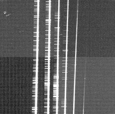
What you see are from left to right the cross-dispersed orders, from Order 3 to Order 8. The short horizontal features are sky lines. The “vertical lines” are the dispersed science target in each order. In the raw data, the red end is at the bottom and blue at the top. This will be reversed when the data is resampled and the distortion corrected and wavelength calibration are applied.

With all the calibrations in the local calibration manager, for a Quicklook Quality output, one only needs to call reduce on the science frames to get an extracted spectrum.

reduce @sci155.lis @nopinhole.param

For a Science Quality output, it is recommended to run the reduction in interactive mode, in particular to adjust the wavelength shift often needed for the telluric correction.

To run the reduction with all the interactive tools activated, set the interactive parameter to True. In this case, the need for interactivity lies mostly in the telluric correction since an offset in wavelength needs to be applied. This is not always needed but it’s safer to verify anyway. To target that step, one would use telluricCorrect:interactive=True instead of the non-specific call that activates all the interactive steps.

reduce @sci155.lis -p interactive=True @nopinhole.param
reduce @sci168.lis -p interactive=True @nopinhole.param
reduce @sci181.lis -p interactive=True @nopinhole.param

When you get to the telluricCorrect step, you can experiment with the shift between the telluric standard and the target. Both need to be well aligned in wavelength to optimize the correction. We find that the following offsets are required: -0.7 for 1.55 ${\mu}$ m, -0.1 for 1.68 ${\mu}$ m, and -0.11 for 1.81 ${\mu}$ m.

(Depending on your interactive adjustments during wavelength calibrations and the calculation of the telluric model, those offsets might be different for you.)

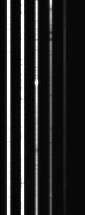
A section of 2D spectrum before extraction is shown on the right, with blue wavelengths at the bottom and the red-end at the top. Note that each order has been rectified and is being stored in separate extensions in the MEF file. Here they are displayed together, side by side. (reduce -r display N20191013S0006_2D.fits -p zscale=False, launch DS9 first.)

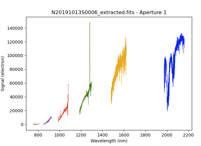
Each order is extracted separately and stored in separate extensions in the MEF file. The 1D extracted spectrum before telluric correction or flux calibration, obtained by adding the option -p extractSpectra:write_outputs=True to the reduce call. You can plot all the orders on a common plot with dgsplot. (The --thin option simply plots a thinner line than the default width.)

dgsplot N20191013S0006_extracted.fits 1 --thin

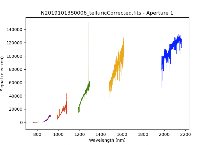
1D extracted 1.55 |um| spectrum before telluric correction or flux calibration

The 1D extracted spectrum after telluric correction but before flux calibration, obtained with -p telluricCorrect:write_outputs=True, looks like this.

dgsplot N20191013S0006_telluricCorrected.fits 1 --thin

1D extracted 1.55 |um| spectrum after telluric correction or before flux calibration

And the final spectrum for one central wavelength setting, corrected for telluric features and flux calibrated.

dgsplot N20191013S0006_1D.fits 1 --thin

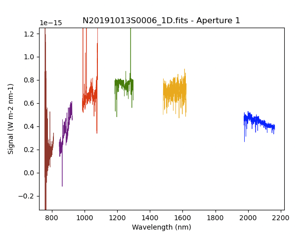
1D extracted 1.55 |um| spectrum after telluric correction and flux calibration

In the final spectrum, the orders remain separated. Here they are simply plotted one after the other on a common plot.

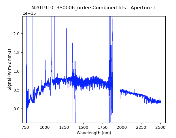
The plots above are for one central wavelength setting. We probably want to scale and stitch all the orders from all 3 final spectra together to get one continuous spectrum. We use the primitive combineOrders to do that.

reduce -r combineOrders N20191013S0006_1D.fits N20191013S0010_1D.fits N20191013S0014_1D.fits -p scale=True

dgsplot N20191013S0006_ordersCombined.fits 1 --thin

Full coverage 1D extracted spectrum after telluric correction and flux calibration

5.2. Example 2 - SXD+111 Point Source - Using the “reduce” command line

5.2.1. The dataset

5.2.2. Configuring the interactive interface

5.2.3. Set up the Local Calibration Manager

5.2.4. Create file lists

5.2.4.1. Three lists for the flats

5.2.4.2. A list for the pinholes

5.2.4.3. Three lists for the arcs

5.2.4.4. Three lists for the telluric

5.2.4.5. A list for the science observations

5.2.5. Bad Pixel Mask

5.2.6. Master Flat Field

5.2.7. Processed Pinholes - Rectification

5.2.8. Wavelength Solution

5.2.8.1. Summary of the Technique for Science Quality

5.2.8.2. Solution from the Arc Lamp

5.2.8.3. Solution from Sky Emission Lines

5.2.8.4. Verifying the Solutions with fitTelluric

5.2.8.4.1. For 1.55 m

5.2.8.4.2. For 1.68 m

5.2.8.4.3. For 1.81 m

5.2.8.5. Combining orders

5.2.8.6. Cleaning up the Calibration Database

5.2.9. Telluric Standard

5.2.10. Science Observations

5.2.8.4.1. For 1.55 ${\mu}$ m

5.2.8.4.2. For 1.68 ${\mu}$ m

5.2.8.4.3. For 1.81 ${\mu}$ m