7. Tips and Tricks

7.1. Fix Bad WCS

In GNIRS data, it is not uncommon for the World Coordinate System (WCS) values in the headers to be wrong in the raw data. In the step prepare, which every recipes starts with, a primitives called standardizeWCS inspect the coordinates and looks for relative discrepancies between the WCS of the all the files relative to the first one. Correct WCS values are essential to sky association and to the alignment of the frames before stacking.

If the reduction crashes with this message:

"ValueError: Some files have bad WCS information and user has requested an exit"

it means that the WCS values in the headers of at least one file are wrong.

This can be fixed. standardizeWCS can try to fix things. For GNIRS longslit data, using the option -p prepare:bad_wcs=new seems to work reliably. Eg.:

reduce @sci.lis -p prepare:bad_wcs=new

7.2. Get the BPMs

7.2.1. Getting Bad Pixel Masks from the archive

Starting with DRAGONS v3.1, the static bad pixel masks (BPMs) are now handled as calibrations. They are downloadable from the archive instead of being packaged with the software. There are various ways to get the BPMs.

Note that at this time there no static BPMs for Flamingos-2 data.

7.2.2. Manual search

Ideally, the BPMs will show up in the list of associated calibrations, the “Load Associated Calibration” tab on the archive search form (next section). This will happen of all new data. For old data, until we fix an issue recently discovered, they will not show up as associated calibration. But they are there and can easily be found.

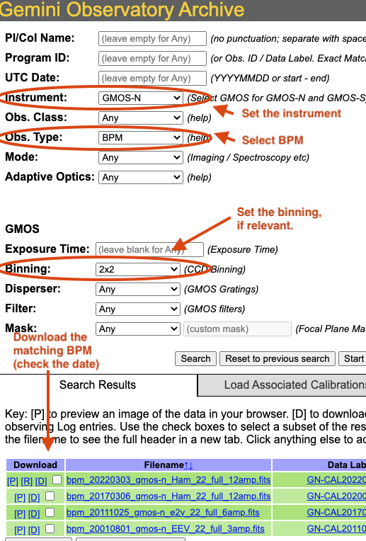
On the archive search form, set the “Instrument” to match your data, set the “Obs.Type” to “BPM”, if relevant for the instrument, set the “Binning”. Hit “Search” and the list of BPMs will show up as illustrated in the figure below.

The date in the BPM file name is a “Valid-from” date. It is valid for data taken on or after that date. Find the one most recent BPM that is valid for your date and download (click on “D”) it. Then follow the instructions found in the tutorial examples.

7.2.3. Associated calibrations

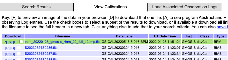
The BPMs are now handled like other calibrations. This means that they are also downloaded from the archive. From the archive search form, once you have identified your science data, select the “Load Associated Calibrations” (which turns to “View Calibrations” once the table is loaded). The BPM will show up with the green background and unlike on the screenshot below, they are now located at the bottom of the primary list.

7.3. Plot a 1-D spectrum

The dgsplot tool can be used to plot and inspect a 1-D spetrum in a matplotlib window. Eg.:

dgsplot N20210407S0173_1D.fits 1

If you want to plot the spectrum in your own Python script, here’s what you can do. This will use the correct WCS as opposed to the approximation stored in FITS headers.

import matplotlib.pyplot as plt
import numpy as np

import astrodata
import gemini_instruments

ad = astrodata.open('N20170113S0146_1D.fits')
ad.info()

fig, ax = plt.subplots()
for ext in ad:
    w = ext.wcs(np.arange(ext.data.size))
    ax.plot(w, ext.data, lw=0.5)

units = ad[0].wcs.output_frame.unit[0]
plt.ylim(0, np.max(ad[0].data) * 1.5)
plt.xlabel(f'Wavelength ({units})')
plt.ylabel(f'Signal ({ad[0].hdr["BUNIT"]})')
plt.show()

7.4. Inspect the telluric model

The telluric model is stored in the processed telluric star file. To inspect the telluric model, you can use the following Python code.

import numpy as np
import matplotlib.pyplot as plt

import astrodata
import gemini_instruments

ad = astrodata.open('N20210407S0188_telluric.fits')
w = ad[0].wcs(np.arange(ad[0].data.size))
plt.plot(w, ad[0].TELLABS)
plt.show()

7.5. Inspect the sensitivity function

The sensitivity function is stored in the processed telluric star file. To inspect the sensitivity function, you can use the following Python code. The example below plots the sensitivity function for the first of six orders, ad[0], which is Order 3. To plot Order 8, you would use ad[5].

import numpy as np
import matplotlib.pyplot as plt

import astrodata
import gemini_instruments

from gempy.library import astromodels as am

ad = astrodata.open('N20210407S0188_telluric.fits')
sensfunc = am.table_to_model(ad[0].SENSFUNC)
w = ad[0].wcs(np.arange(ad[0].data.size))

std_wave_unit = ad[0].SENSFUNC['knots'].unit
std_flux_unit = ad[0].SENSFUNC['coefficients'].unit

plt.xlabel(f'Wavelength ({std_wave_unit})')
plt.ylabel(f'{std_flux_unit}')
plt.plot(w, sensfunc(w))
plt.show()

7.6. Useful parameters

7.6.1. skip_primitive

I might happen that you will want or need to not run a primitive in a recipe. You could copy the recipe over and edit it. Or you could invoke the skip_primitive parameter to tell DRAGONS to completely skip that step.

Let’s say that you want the data aligned but not stacked. You would do:

reduce @sci.lis -p stackFrames:skip_primitive=True

7.6.2. write_outputs

When debugging or when there’s a need to inspect intermediate products, you might want to write the output of a specific primitive to disk. This is done with the write_outputs parameter.

For example, to write the extracted spectrum before it is corrected for telluric features and flux calibrated, you would do:

reduce @sci.lis -p extractSpectra:write_outputs=True